EN 10211:2007 defines a procedure for validating software for thermal bridge calculations. The workflow is structured in Annex A for two different two-dimensional simulation cases. As described below, the DELPHIN software can be used as a program for two-dimensional, transient thermal and moisture simulations for calculating the cases.
If DELPHIN is to be used for stationary state calculations, constant boundary conditions are applied. The simulation should run until changes resulting from the initial conditions disappear and constant processes occur. Therefore, the selection of initial conditions has an impact on the simulation duration.
We recommend starting with a short simulation time of a few hours to 2 days, using hourly output values. If the displayed variables are still changing, we can extend the simulation time by a factor of 2 or 3 (depending on the extent of the deviation) and continue the simulation. Normally, even complex designs reach a steady state within a few simulation days.
In the simulations for the EN 10211:2007 validations, we sometimes need simulation times of over 40 days (which says a lot about the probability that a steady-state situation can even be achieved in real life).
Validation case 1
This surface case uses the symmetry of the component in the calculation. The outputs should be determined at defined grid points.
In DELPHIN, we use a modeling trick to generate the grid. We define two materials with the same properties but different names. We create a checkerboard pattern with these materials. Now we can use the built-in grid generator, set the minimum element thickness and the expansion factor, and generate the required grid.
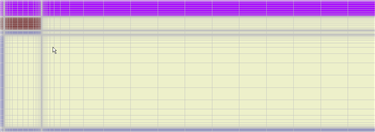
The generated grid is shown in the graphic below.
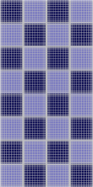
Das ist das generierte Gitter mit einer Elementdicke von 1mm, einen Ausdehnungsfaktor von 1.476 und einer Elemtanzahl von 15488.
Validation results and project
The finished project, which we used for validation, can be downloaded via the link below. It has been tested in versions 5.6.4 and 5.6.5. The next DELPHIN has already integrated the two cases as examples.
EN_ISO_10211_2007_Case1.dpj
(EN_ISO_10211_2007_Case1.dpj)
The calculated results are shown in the following tables with the original values and the deviations that occurred. All deviations are below the limit value of 0.1 Kelvin.
The first table contains the results calculated using the DELPHIN simulation program. The values in brackets are reference values for comparison.
9.659 (9.7)   13.385 (13.4)   14.736 (14.7)   15.093 (15.1)
5.249 (5.3)    8.643  (8.6)   10.320 (10.3)   10.815 (10.8)
3.186 (3.2)    5.610  (5.6)    7.017  (7.0)    7.468  (7.5)
2.012 (2.0)    3.641  (3.6)    4.660  (4.7)    5.002  (5.0)
1.261 (1.3)    2.308  (2.3)    2.987  (3.0)    3.219  (3.2)
0.739 (0.7)    1.359  (1.4)    1.767  (1.8)    1.908  (1.9)
0.341 (0.3)    0.629  (0.6)    0.819  (0.8)    0.886  (0.9)
The following table shows the deviations of the calculations from the given values.
0.04	0.02	0.04	0.01
0.05	0.04	0.02	0.01
0.01	0.01	0.02	0.03
0.01	0.04	0.04	0.00
0.04	0.01	0.01	0.02
0.04	0.04	0.03	0.01
0.04	0.03	0.02	0.01
Grid sensitivity study
Grid sensitivity studies are performed to quantitatively estimate numerical errors that are introduced into the results by the type and shape of the calculation grid. This allows the effects of various grid generation parameters that significantly influence the density of the numerical grid to be investigated. In our two cases, we investigate the effects of a change in the grid on the calculated temperature distributions in the component. To do this, we change the minimum element thickness and the stretch factor, and thus also the number of elements. These are the decisive factors for significantly influencing the component grid and investigating the effects.
One of the varied parameters is the stretch factor. It specifies the size ratio of two adjacent elements and thus the expansion of the grid. The other describes the minimum thickness of the elements at the edge or at material boundaries. By specifying the two parameters, the maximum element thickness is calculated automatically, provided that no upper limit is specified. In the first two diagrams, one of these two parameters is varied while the other remains the same. In the third case, we examine the extent to which the calculation results improve when the change in both parameters leads to a steadily finer grid.
The abscissa axis of the diagrams shows the number of elements, the minimum thickness of the elements, and the stretch factor for the various cases. The ordinate axis shows the difference between the calculated temperatures and those specified in the standard. The six most significant points were selected from the 28 calculated points for the component and are shown in the diagrams.
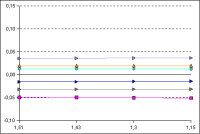
The stretch factor varies in these diagrams from 1.15 to 1.51. The minimum element width was always set to 1 mm. The straightness of the lines shows that the stretch factor has no significant influence on the results.
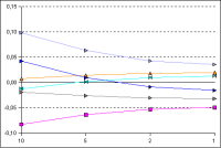
The parameter for the minimum width/height of the grid elements at the edge was changed in the range from 1 mm to 10 mm, while the stretch factor remained constant at 1.51. It can be seen that the element size at the edge or at material boundaries has a significant influence on the results. In particular, it can be seen that with larger edge elements and thus a smaller number of elements, the calculated temperatures deviate more strongly from the given temperatures. If the grid elements at the edge are reduced in size (smaller minimum element thickness), the grids become finer and the deviations decrease.
With a minimum element thickness of 1 mm, further reduction of the edge elements in this test case only results in a slight improvement in the results. It can therefore be assumed that the results have been determined with sufficient accuracy.
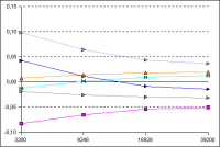
The stretch factor is changed from 1.51 for the coarsest grid to 1.21 for the finest grid. At the same time, the minimum element width is reduced from 10 mm to 1 mm.
The following table shows the cases considered and the respective number of elements in the calculation grid.
Case Elements min stretch
I 3200 10 1,51
II 9248 5 1,3
III 16928 2 1,3
IV 39200 1 1,21
The results are almost identical to those shown in the diagram for the minimum element thickness. It is therefore more important to calculate with a small element thickness at the edge than to create optically finer grids using small stretch factors. The latter leads to more elements and longer calculation times, but hardly any increase in accuracy.
However, in transient simulations, especially when moisture transport is taken into account, strong gradients can also occur inside the component. An example of this would be a simulation of a water absorption test. Here, the stretch factor becomes important again!
Validation case 2
Dieser Validierungsfall stellt die Berechnung eines zweidimensionalen Details dar, welches aus Beton, Holz, Wärmedämmung und Aluminiumblech besteht.
The design was modeled as shown in the image on the right. Thin metal sheets usually require a very fine grid around and close to the sheet layers. Narrow elements close to the surface are also needed to capture the heat flow.
In addition, the large differences in the thermal conductivity of the materials lead to longer calculation times. Nevertheless, even with a very detailed grid, the calculation is completed within 3 minutes on a normal PC.
The next graphic shows the simulation model without discretization.

Now, a coarse discretization for the second case with only 6460 elements is shown.
The first table contains the results calculated using the DELPHIN simulation program. The values in brackets are reference values for comparison.
A: 7.125 (7.1) 0.025
B: 0.763 (0.8) 0.037
C: 7.967 (7.9) 0.067
D: 6.331 (6.3) 0.031
E: 0.829 (0.8) 0.029
F: 16.384 (16.4) 0.016
G: 16.249 (16.3) 0.051
H: 16.747 (16.8) 0.053
I: 18.328 (18.3) 0.028

Total heat flux: 9.534 (9.5) W/m
heat flux difference: 0.034 W/m
Grid sensitivity study
In this case, a grid sensitivity study was also performed. The results are shown as examples for selected points. A calculation was performed for each grid variation. Variation studies have shown that, here too, the stretch factor has no significant influence on the results. Thus, in the following discussion, only the minimum element thicknesses at the edge are considered, and all grid variants are generated with a stretch factor of 1.51.
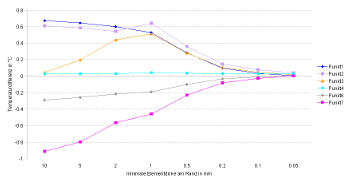
The minimum element thickness in mm is plotted on the x-axis, and the y-axis shows the temperature differences (relative to the reference temperatures) at selected sensor points in K. The minimum element thickness plays a very important role in mesh generation, as the component is traversed by a highly heat-conductive aluminum sheet, which has a major influence on the temperature distribution. Therefore, a very fine mesh must be selected in the area where the sheet is located in order to obtain the most accurate results possible. For this reason, the minimum element thickness at the edge or at material layer boundaries was varied between 10 mm and 0.05 mm. As can be easily seen in the diagram, the results below 0.2 mm no longer change significantly, whereas from 10 mm to 0.5 mm there are sometimes drastic differences in the calculated temperatures for individual points.
The strong influence of the element thickness at the edge or at component boundaries on the accuracy of the result can be explained by the numerical implementation of the boundary condition. In the control volume method used in DELPHIN, a single state is defined for each element. This means that no distribution of conservation quantities within the element is described. The temperature at the edge of the element is therefore assumed to be the same as at the center of the element. In the case of strong temperature gradients at the edge, this leads to an error that is directly proportional to the element size at the edge. Therefore, small grid elements should always be used in areas with strong temperature gradients.