1. Overview
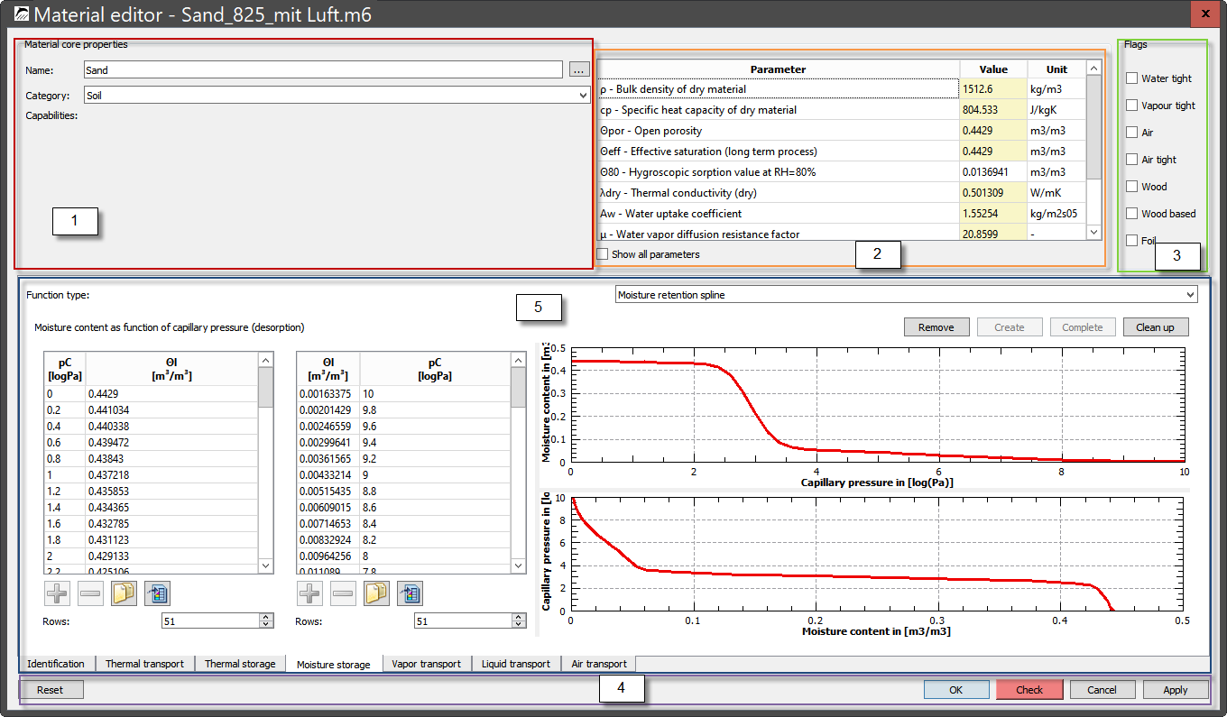
The main window can be divided into five areas as shown in Figure 1.
-
Basic data with material name
-
Basic parameters
-
Flags
-
Buttons
-
Model view
The basic data, the basic parameters and the flags are always visible. The displayed model view depends on the section and model selection. Sections here are sections of the material file, which are assigned to certain physical processes, for example. The division in the editor is slightly different from the material file for reasons of overview. The following sections can be selected:
-
Identification - further texts and dates
-
Heat transport
-
Heat storage
-
Moisture storage
-
vapour transport
-
Liquid water transport
-
Air transport
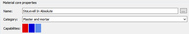
1.1. Basic data
This area displays the material name, material category and transport capabilities (color-coded).
The material name, like all other descriptions, can be specified in several languages. In the main view, the texts are always displayed in the language of the operating system. If this language is not available, the text is displayed in English.
To edit the text in the other languages you should click the button with 3 dots on the right. Then a corresponding editor will open.
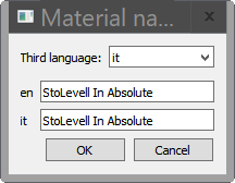
In this dialog the text can be entered directly in English, the language of the operating system and another language. The third language can be selected in the selection box above. The default language is Italian. If English is the language of the operating system only two languages will be shown.
The category can be selected from one of 13 types:
-
Coatings
-
Plaster and mortar
-
Building bricks
-
Natural Stones
-
Concrete-containing building materials
-
Insulating materials
-
Building boards
-
Timber
-
Natural materials
-
Soil
-
Cladding panesl and ceramic tiles
-
Foils and waterproofing products
-
Miscellaneous
The transport properties are displayed in color-coded form. A particular transport type can only be taken into account if all the necessary properties are available. Furthermore, this special transport must not be switched off by using a flag (section Identification). The colors have the following meaning:
- Red
-
Heat transport
- dark blue
-
Liquid water transport
- blue
-
Vapour transport
- light blue
-
Air transport
The transport processes for salt and VOC are currently not supported by the material editor.
1.2. Basic Parameters
The basic parameters represent a selection of data which on the one hand should help to select a concrete material from the database and on the other hand can serve as parameters for transport and storage models. Some parameters are derived from the models themselves. These cannot then be changed directly. A description of all basic parameters can be found in the following table. In column 'Usage' one can find the transport and storage processes which are influenced by this parameter. If nothing is entered there, the parameter serves only for information and is not used in the simulations!
| Size | Unit | Description | Usage |
|---|---|---|---|
ρ |
kg/m3 |
bulk density of dry material |
heat storage |
cp |
Ws/kgK |
specific heat capacity |
heat storage |
Θpor |
m3/m3 |
porosity |
moisture storage, vapour transport, air transport |
Θeff |
m3/m3 |
effective saturation |
moisture storage, heat conduction, liquid water transport |
Θcap |
m3/m3 |
capillary saturation |
- |
Θ80 |
m3/m3 |
moisture content at 80% relative humidity |
- |
λdry |
W/mK |
thermal conductivity of the dry material |
heat transport |
Aw |
kg/m2s0.5 |
water absorption coefficient |
liquid water transport |
μ |
- |
water vapour diffusion resistance factor dry |
vapour transport |
sd |
m |
diffusion equivalent air layer thickness |
vapour transport (vapour retarders) |
Kleff |
s |
liquid water conductivity for pressure gradient |
liquid water transport |
Dleff |
s |
liquid water conductivity for water content gradient |
liquid water transport |
Kg |
s |
air permeability |
air transport |
λdesign |
W/mK |
design value of the thermal conductivity |
heat transport with purely thermal calculation |
αT |
1/K |
linear thermal expansion coefficient |
- |
αH |
- |
hygric expansion coefficient (volumetric moisture content) |
- |
The material database format of DELPHIN supports even more basic parameters, but these are not supported by the editor. You can find more information here: https://nbn-resolving.org/urn:nbn:de:bsz:14-qucosa-126274
The following figure shows the section of the editor for the basic parameters.
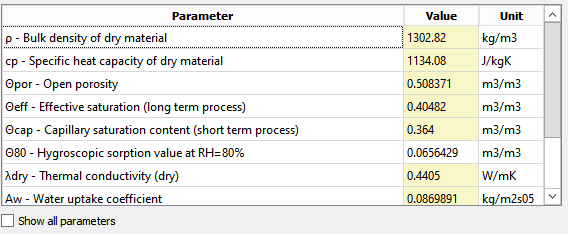
By checking the box 'Show all parameters' all possible parameters (see table) are displayed in the list, otherwise only those with a valid value are shown. If a number is marked yellow there, you can change this number. Some values can also be deleted. But this is only possible if this parameter is no longer needed (flags, models). You delete a parameter by deleting the value and then pressing ENTER. If this value cannot be deleted, the original value is re-entered.
1.3. Flags
The flags are located to the right of the basic parameters.
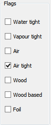
These have different effects and can be grouped as follows:
Transport flags:
-
Water tight - liquid water transport switched off (keyword: WATER_TIGHT)
-
Vapour tight - vapour transport switched off (keyword: VAPOR_TIGHT)
-
Air tight - air transport switched off (keyword: AIR_TIGHT)
If such a flag is set, the respective transport is no longer possible and all related parameters and models are no longer used (and can be deleted). If a material is both water tight and vapour tight, no parameters for moisture transport and storage is required. This is the case for materials such as glass, metals or solid plastics. The corresponding keywords for the material files are listed in brackets.
Material flags:
-
Air - The material is air. Moisture storage function is provided internally and does not need to be specified (keyword: AIR)
-
Wood - The material is wood. For information only (keyword: WOOD).
-
Wood based - The material is wood. Informative only (keyword: WOODBASED).
-
Foil - The material is a vapour barrier. An sd-value must be given.
1.4. Buttons
There are five buttons on the bottom of the material editor. These have the following effect:
1.4.1. Reset
Here the current material file is read in again from the database and the editor is set to these values. This overwrites all unsaved changes.
1.4.2. Ok
A click on this button saves the material file with the current contents of the editor and closes the editor.
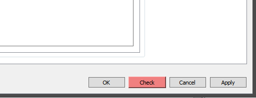
1.4.3. Check
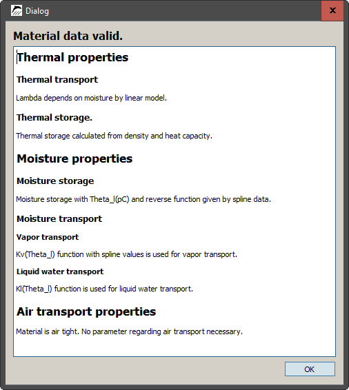
This button performs a check of the current status of the material. All models and basic parameters are checked and a description of the status is provided.
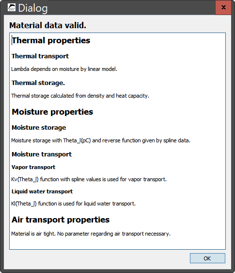
The figure above shows the output for a valid record. The status and the models used are displayed for each section. This button is also used to indicate if there are problems in the data set:
-
yellow marking - data set valid, but warnings present
-
red marking - data record invalid
The following two figures show the behavior in case of an invalid data set.
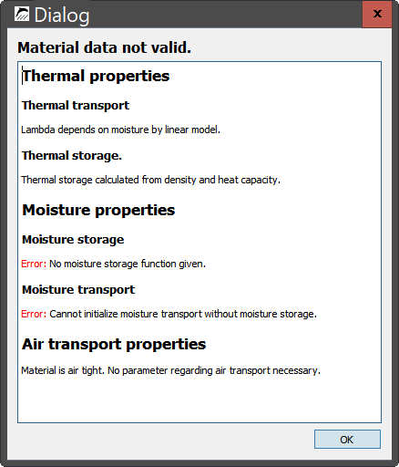
When you click on the Check button, the check window is displayed, showing the cause of the invalid record.
1.4.4. Cancel
Closes the editor without saving the data set.
1.4.5. Apply
Saves the data set without closing the editor.
1.5. Model view and section selection
The appearance of the model view depends on the selected section. The currently available sections are shown in [Main_Window_Sections]. The individual sections are described below.
1.5.1. Identification
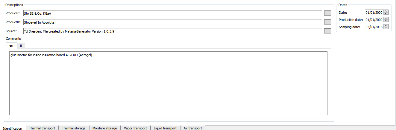
The figure above shows the identification area. Here the name of the manufacturer, the product designation, the data source and comments can be specified. The language selection is done as described in [Basic_data]. The comment is only available in German, English and Italian or in case of an english operating system only in English and Italian. Other languages must be entered directly into the material file using a text editor. Additionally, there are date specifications on the right. These have the following meaning:
-
Date: when the data record was created
-
Production date: when was the measured material produced
-
Sampling date: when were the measured samples prepared
If 01/01/2000 is entered as the date, this date is not known.
If further specifications are to be made in the identification area, this must be done directly with a text editor in the material file.
1.5.2. Models - General
All following model sections have a similar structure.
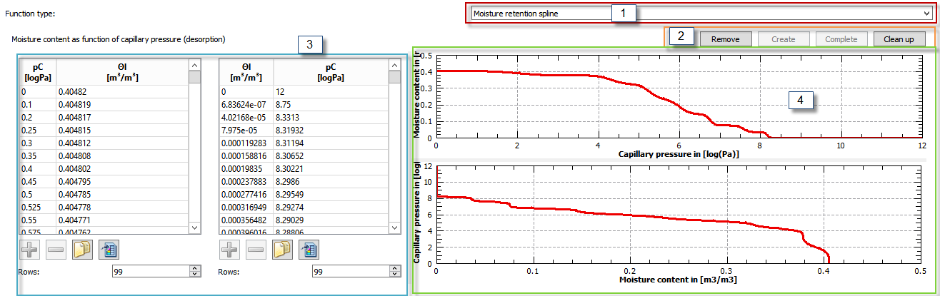
The figure above show a view for general models. This is divided into four areas:
-
Model selection
-
Buttons Model Editing
-
Tables for data values
-
Graphical representation
Model selection (1)
Here is a selection box with which you can choose a model from the available ones. Only the models of the selected section are available. For all sections there is also a point No model. This is selected if nothing is specified for this section. For sections with only one possible model, the selection box is replaced by two radio buttons (heat storage).
Buttons model editing (2)
There are three buttons at the top right. These are shown in each model, but not always available.
Remove deletes the currently selected model.
Create inserts data for the selected model.
Complete is only available for incomplete models and fills the data gaps.
Clean deletes all other data from this range except the data required for the selected model. This can be used to remove old models that are no longer needed.
Tables for data values (3)
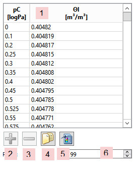
The data table (1) shows the currently used data. For models created from the basic parameters (linear), this table is grey and the values cannot be changed. Otherwise all values can be changed. The decimal separator must always be that one which the operating system used. If an input cannot be interpreted as a numerical value, the background will turn red.
Button 1 (plus) allows to add a value pair above the current selection. The mean values of the upper and lower data are entered as default. Button 2 (minus) deletes the selected data row. However, at least two value pairs must remain in the table. Delete is deactivated when this limit is reached. A click on button 4 replaces the content of the entire table with the content of the clipboard. The data for this must be arranged in such a way that each row contains a pair of values (separated by a tabulator). The decimal separator must be that of the operating system. If the contents of the clipboard cannot be used, nothing happens. With button 5 the content of the table is copied into the clipboard and is available for editing with external programs. In the input field 6 the number of lines of the table can be changed. The values are always added or deleted at the end. Here too, the minimum number is 2 pairs of values.
Graphical representation (4)
In this area the available data is displayed graphically. Changes are not possible here. Exporting the display and adjusting the charts is also not possible with the current version. If you need your own view, you can export the data to the clipboard and then display it using a tool of your choice.
1.5.3. Heat transport
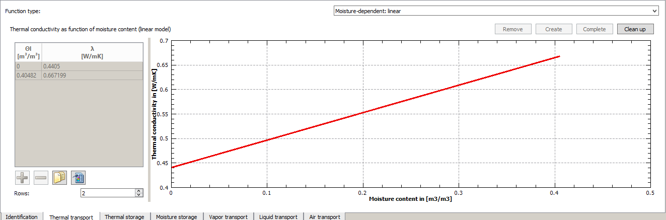
The figure above shows the view for the Heat Transfer section. The first view always shows the currently selected model. The following models are available for heat transport:
-
Moisture dependent: linear
-
Moisture dependent: spline
-
Temperature dependent: spline
If no model is available, 'No model' would be displayed in the selection box. In case of heat transport, this would mean that the material is not valid (usable) because heat transport is always required. In the following the individual models are described:
Moisture dependent: Linear
This model consists of a simple linear dependence of the thermal conductivity on the volumetric moisture content. The thermal conductivity of water is used as the slope (0.6 W/mK). Thus a simple parallel approach of the heat flows in material and pores is represented. The thermal conductivity of the dry material from the basic parameters is the only parameter required. If this value is changed, the model adapts automatically. Since only one basic parameter is needed here, this model should always be possible or available. Therefore this model cannot be removed. If its still missing, the thermal conductivity is not given for the base parameters.
Moisture dependent: Spline
Here the moisture dependence is represented by data pairs for the volumetric moisture content in m3/m3 and the thermal conductivity in W/mK. Linear interpolation is performed between these points. Such data pairs are also used for many other models.
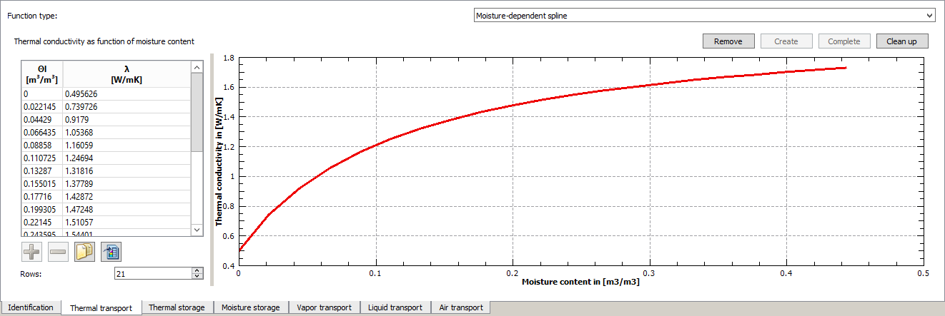
The value for the moisture content of 0 m3/m3 should correspond to the thermal conductivity in the basic parameters. A change of the base value has no influence on this data.
Temperature dependent: Spline
This section works analogous to the previous one. The temperature in °C and the thermal conductivity in W/mK must be entered here as value pairs. This model can be given parallel to the moisture-dependent data. Both dependencies are then considered. There are two prerequisites:
-
The moisture-dependent thermal conductivity is defined for 23°C.
-
The temperature-dependent heat conductivity is defined for 0 m3/m3.
1.5.4. Heat storage
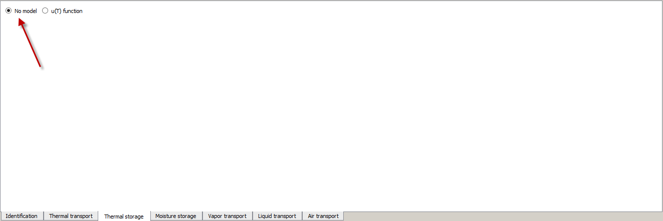
By default, the heat storage is calculated based on the basic parameters density and heat capacity. The moisture content or the stored heat of all three phases (vapour, water, ice) is taken into account internally. It is possible to use a function u(T) as a function of the internal energy depending on the temperature instead. In the current DELPHIN version, this is only possible with pure heat transport. If the moisture transport is switched on, DELPHIN uses the standard model instead. This is also the case if a u(T)-function exists. The main application of such a function is the modeling of PCMs. For questions about this, please contact the developers.
1.5.5. Moisture storage
A model for moisture storage is required as soon as a moisture flow is to be calculated, i.e. the material is not vapour and water tight.
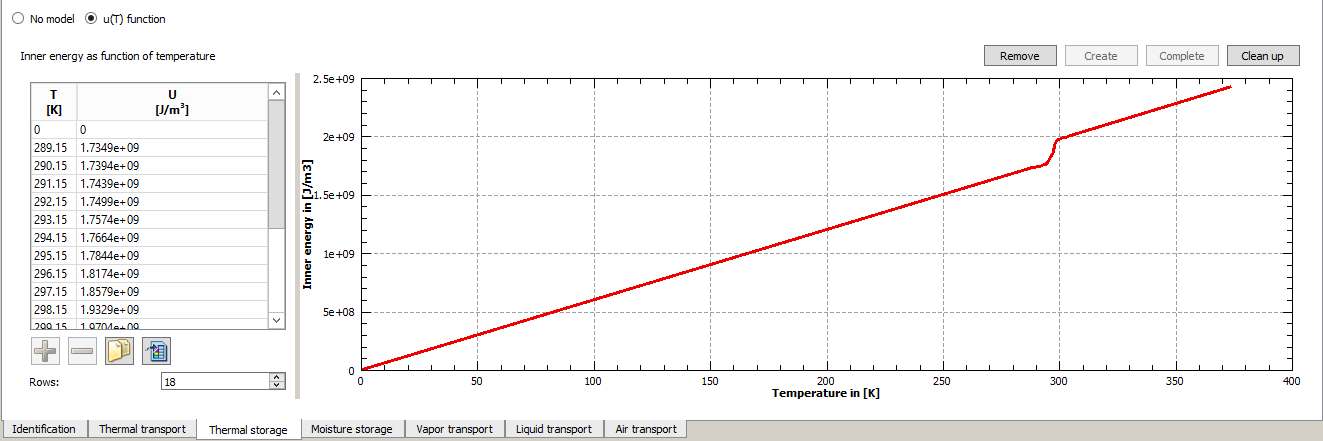
The standard model for moisture storage is the **MoistureRetentionCharacteristic (MRC). Here, the water content is represented as a function of capillary pressure. In DELPHIN, the decadic logarithm of the negative capillary pressure (pC) is used instead of the capillary pressure itself. So that the DELPHIN solver can calculate quickly, the corresponding inverse function should always be given (right table). If this is not available, there are several possibilities:
-
You use the data set as it is and let DELPHIN calculate the inverse function. This is not recommended because it can lead to numerical difficulties.
-
If the inverse function is missing, the Complete button is active. A click on it creates an inverse function by simply swapping the data pairs. This can also lead to numerical problems during the calculation.
-
Based on the original function, data pairs are generated for both functions. This requires knowledge of the raw data or the original functions used. This is numerically most stable.
The only other model possible is the use of a sorption isotherm.
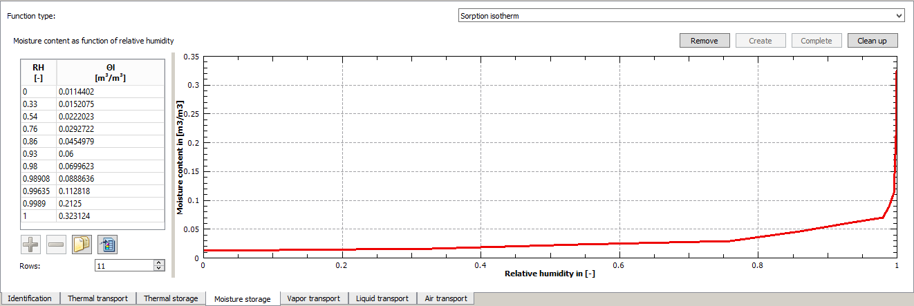
Since a sorption isotherm cannot correctly represent the high moisture range, this function is not recommended for materials that absorb large amounts of moisture (condensation, water contact, rain).
Vapour transport
For vapour transport, a moisture content dependent vapor conductivity (Kv) is generally required. There are three possible models:
-
Kv moisture-dependent: linear
-
Kv moisture-dependent: Spline
-
μ depending on relative humidity
These models are only used if the flag Vapour tight is not set.
Kv humidity dependent: linear
Here the vapour conductivity is considered to be linearly dependent on the moisture content. The value at a moisture content of 0 m3/m3 is calculated from the μ-value of the dry material. The vapour conductivity then drops to 0 when the material is completely saturated (porosity). As parameters, this model requires only the μ-value and the porosity from the basic parameters. This model can neither be deleted nor added. It exists automatically if both base parameters are present. However, it is only used if no other model is available.
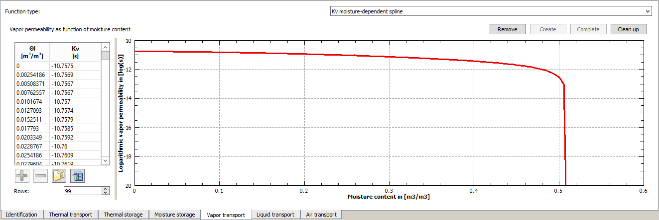
Kv moisture-dependent: Spline
The decadic logarithm of the vapour conductivity Kv is provided as specified data pairs as a function of the volumetric water content. Linear interpolation is performed. The figure above show such a function. The function starts at a moisture content of 0 m3/m3 and ends at porosity. If the porosity changes, the function is adjusted (scaled). The same applies to a change of the μ-value. Here a new Kv-value for the dry material is calculated and the function is adjusted. This model can also be used to generate a moisture-independent vapour conductivity. In this case only two data pairs with the same Kv and the moisture contents 0 and porosity have to be specified (see example 3).
μ depending on the relative humidity
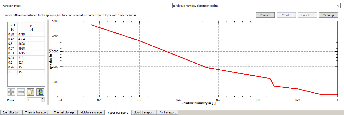
This approach is primarily used for moisture-adaptive vapour retarders (smart vapour retarder). In this case it must be noted that the μ-value specified there applies to a 1 mm thick layer. In the end result, the entire layer has the sd value of the corresponding vapour retarder. This model can be changed by directly entering the data. Furthermore it depends on the μ,-value as well as on the sd-value of the basic parameters. Changing either value will also change this function. If both data are given, the regular layer thickness is also known. It is usually given in the comment to the material.
1.5.6. Liquid water transport
There are two models for liquid water transport, both specified via data pairs. The models differ only in the way the transport is modeled.
-
Kl(Θl) - conductivity for capillary pressure gradient
-
Dl(Θl) - conductivity for water content gradient
The picture below shows as an example the preferred Kl.
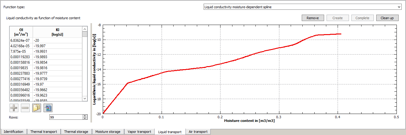
For the data, the conductivity must again be given as a decadic logarithm.
As with vapour transport, a model is only used here if the flag Water tight is not set. If it is set, all models including the associated base parameters can be deleted without invalidating the data set.
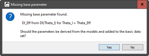
For both models there is a parameter for conductivity at saturation in the base parameters (Kl_Eff and Dl_Eff). Furthermore, a water absorption coefficient (Aw) can exist there. If this and the conductivity parameter are given, a mathematical relationship can be derived. This allows function to be adjusted (scaled) by changing the Aw value. If the Aw-value does not exist, a warning is given. It is then possible to determine this value by simulating the water absorption test. If the material editor is started and it is determined that a transport function exists but the corresponding basic parameter is missing, the possibility is offered to derive this value from the function and enter it.
1.5.7. Air transport
Here a moisture-dependent air permeability is provided. There are two models:
-
Kg moisture dependent: linear
-
Kg moisture dependent: spline
In the linear model, the permeability for the dry material is taken from the basic parameters (Kg). This value then goes linearly towards 0 at complete saturation (porosity). The other model allows the input of data pairs. In contrast to most other models, Kg is not given logarithmically. As with vapour and water transport, an air transport model is only used if the material is not marked as Air tight.
2. Examples
2.1. Hydrophobing of a brick
In this example we are dealing with an internally insulated brick wall. In such a construction, the impermeability to driving rain plays a major role. If this is not the case with the original construction, it must be provided subsequently. In the case of a brick-faced façade, a hydrophobic coating is often applied.
What does hydrophobicity mean for the material? Ideally, the liquid water conductivity should be reduced without affecting the vapour transport. A hydrophobing agent, e.g. on a silicone basis, can be used here, which is applied to the outside of the facade. It penetrates several millimetres deep and changes the liquid water transport there. In Delphin, this can be modelled in such a way that an adapted brick material is used for an approx. 5 mm thick outer layer. How do you proceed?
-
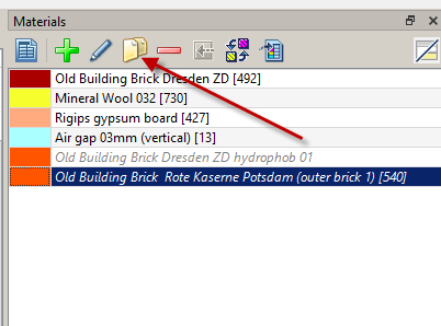
Copy the existing brick material in the material selection
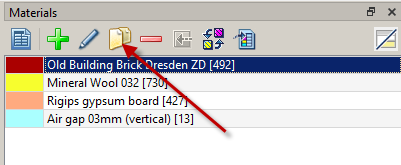
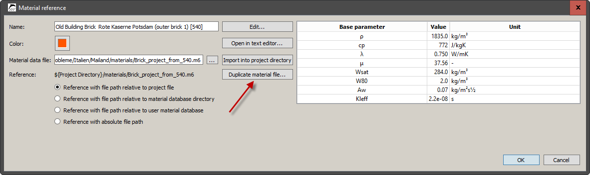
After clicking on the copy button marked with the arrow, the following dialog appears
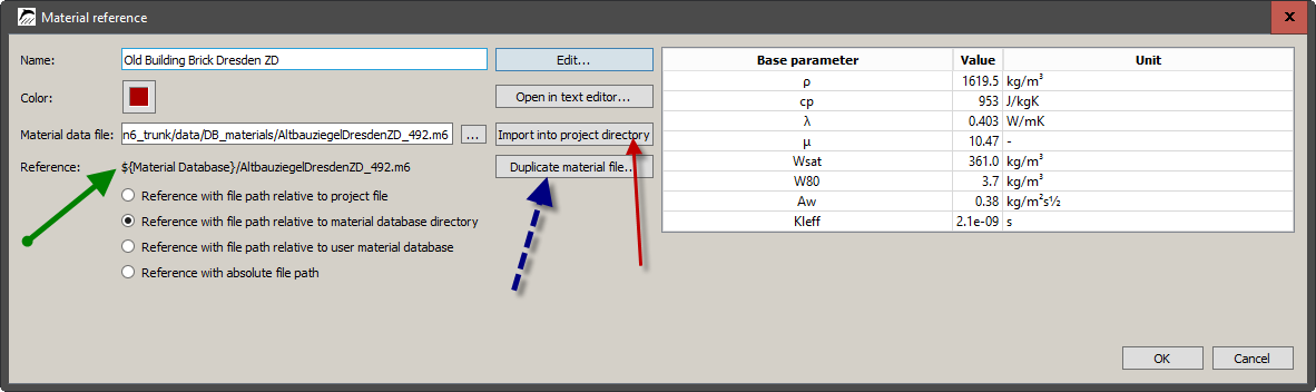
The chosen material was in the DELPHIN material database, which can be easily recognized by the reference (green arrow) that refers to the Material Database. To be able to change the material, it has to be copied. There are two possibilities for this:
-
Copy to the project directory (red arrow)
-
Duplicate material file (blue arrow)
The first button is used to copy material files from the database to another directory. The most suitable directory for this is materials in the project directory. This should be used here as well.
The second button is used to duplicate material files that are already outside the database. This is useful if you want to perform variant studies with several adapted materials.
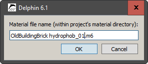
After clicking the first button, another dialog appears:
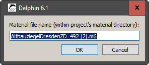
Here you can enter a new name for the new material. By default, a number in square brackets is appended to the existing name. We change the name so that a hydrophobicity can be recognized.
After closing this dialog, you will return to the original dialog. Here you should change the display name and also the color to differentiate to the original material. Then you can close the dialog.
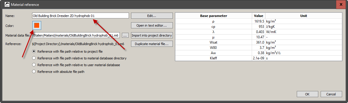
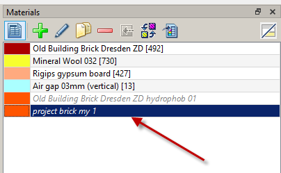
As a result, a new material can now be seen in the material list of the project.
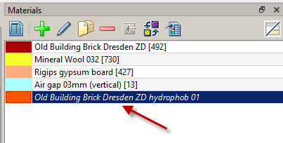
The material is still shown in grey italics because it has not yet been assigned to the construction. Next, the liquid water conductivity has to be adjusted. To do this, open the material reference dialogue again by double-clicking on the material and then click the Edit button. The material editor opens. Here you select the Liquid Water Transport tab.
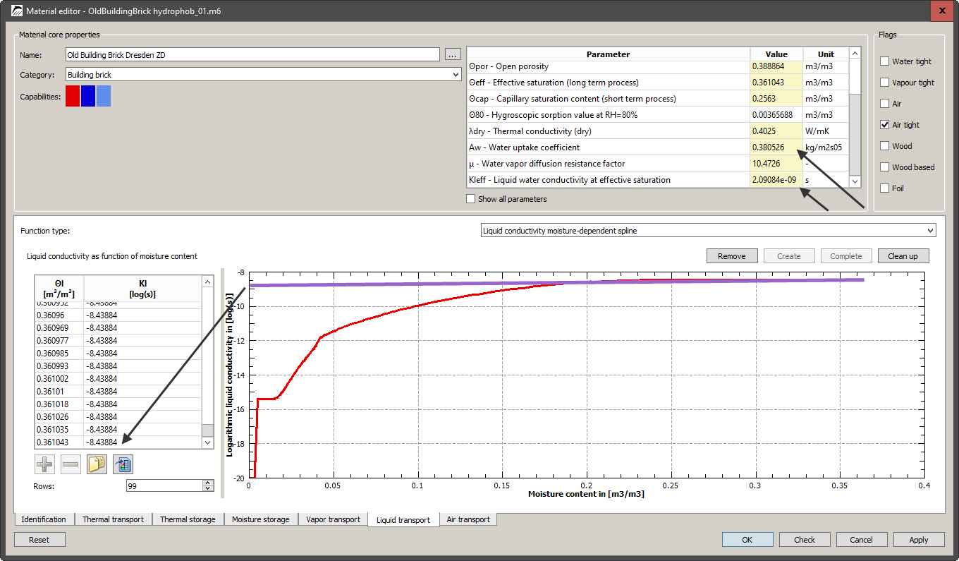
The picture shows the currently used guiding function. This brick has a Kl(Θl) function with a highest Kl value of -8.44log(s). In the basic data there is an Aw-value of 0.38kg/m2s0.5 and a Kl_Eff of about 2*10-9 s. A good hydrophobicity should reduce the Aw-value to at least a tenth (better to a hundredth) of the original value. We now change the Aw-value to 0.01 kg/m2s0.5. All we have to do is double click on the value in the table, adjust it and then press ENTER. The whole function is then scaled down. The result is shown in the following picture:
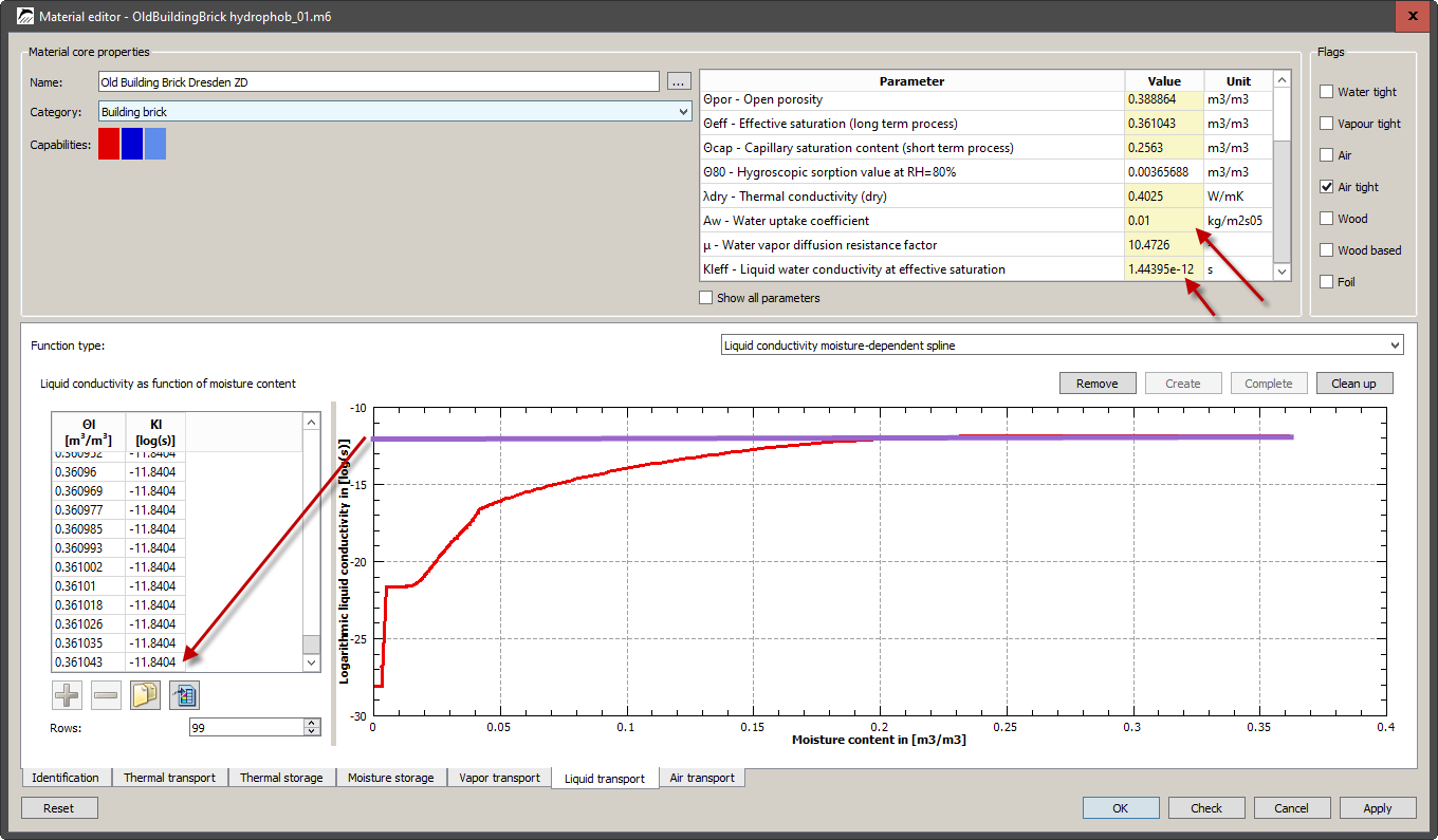
As you can see, not only the Aw-value has changed, but also Kl_Eff, as well as the whole leading function. This material can now be accepted by clicking on Ok and then assigned to the construction.
2.2. Existing material of a building is not in the database
When examining existing buildings, it often happens that the materials used there are not available in the DELPHIN database. Nevertheless, you still need the material characteristics so that you can calculate. Here, there are two procedures:
-
Complete measurement: you take some samples and send them to a qualified laboratory. There, all parameters necessary for the calculation are determined. This is very accurate, but also expensive and time-consuming.
-
Partial measurement - you measure so many parameters that you can identify a material from the database which is as similar as possible to the existing material. The more is measured, the better the result. Then the database material is adapted to the existing material.
In this section variant 2 is to be chosen. A brick is used here as an example. A sample was taken and the following characteristic values were determined:
density: ρ = 1835 kg/m3
Thermal conductivity: λ = 0.75 W/mK
Water absorption coefficient: Aw = 0.07 kg/m2s0.5
The material database is opened in DELPHIN. There, you can choose the category 'Building bricks' and then, by clicking on the column header, sort according to the density. As moisture transport is to be taken into account, the vapour diffusion filter restricts the selection to materials that at least have vapour transport.
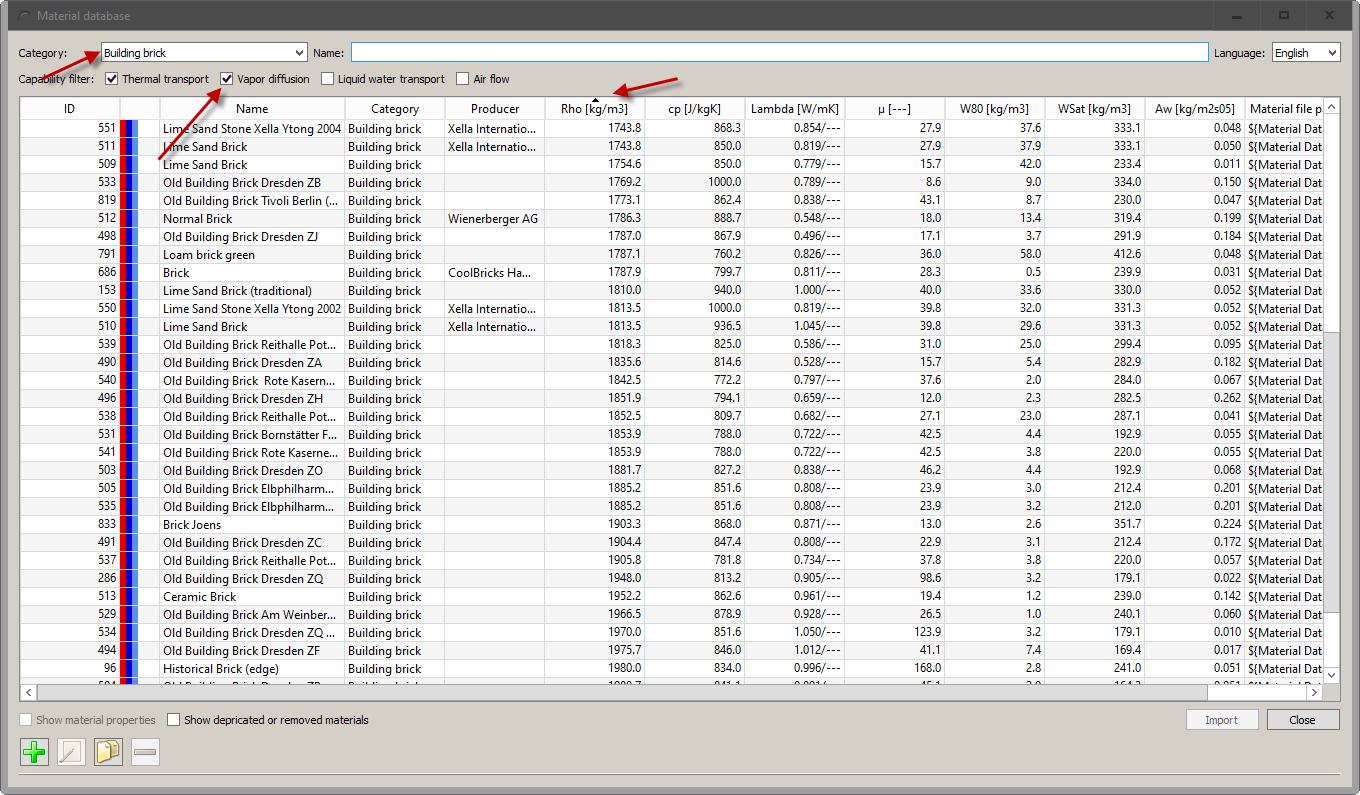
A material with exactly the right data is not included. One should therefore look for similarities. Priority should be given to the Aw-value and next to the thermal conductivity. Although the density is easy to measure, it has only little influence on the calculation result.
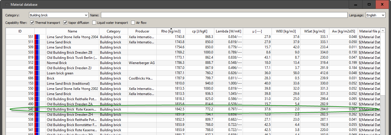
The material with the ID 540 seems to meet the requirements best. Here it would be good to have at least one more measured parameter for moisture (μ-value, Θeff etc.).
Next, the material must be copied so that it can be changed. Here you have two options:
-
Copy to the user database from the material database dialog
-
Importing into the project
A copy into the user database is only useful if this material is needed more often outside of this project. In this case, the material is only needed for the concrete investigation. Therefore point 2 is chosen and the material is imported. For this, select the material and click on Import. Then the material reference dialog will appear:
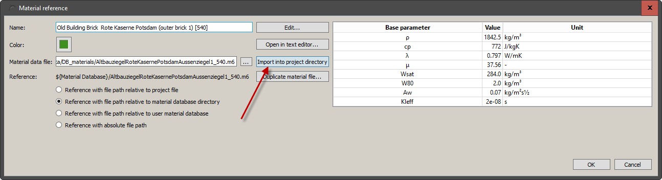
There you click on Import into project directory to save the material in the materials directory of the project.
Afterwards the material database dialog can be closed. The material then appears in the material list of the project. A double click on the material and then a click on Edit in the reference dialog opens the material editor. Here the name should be adapted first. Furthermore, information about measurement and fitting should be entered in the comments.
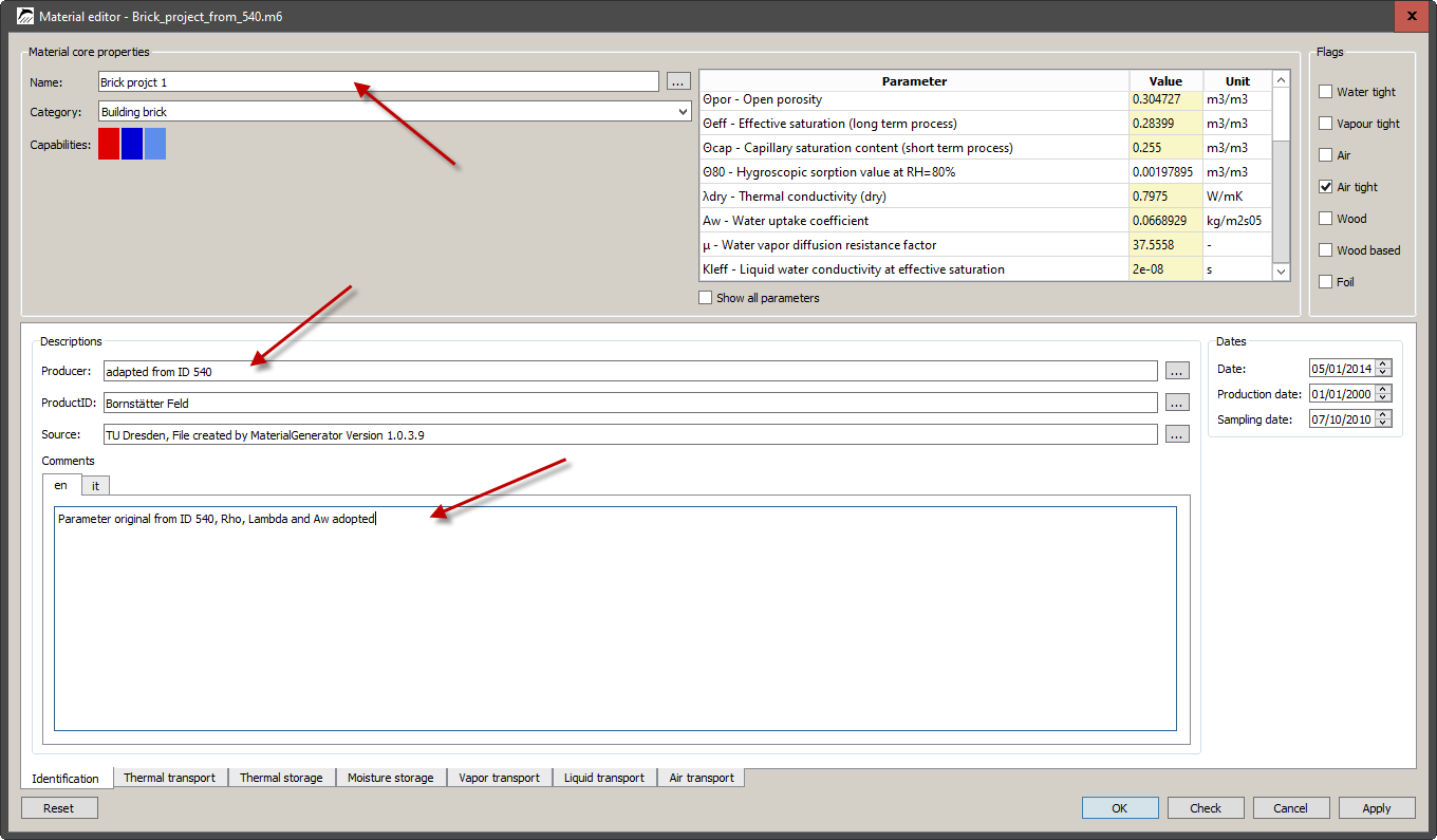
You could also set the date on the right in the identification area to the current date.
Afterwards, the characteristic values must be adjusted. All three measured values are basic parameters and can be changed in the table on the top right. This can lead to side effects in the models:
- Density
-
influences the heat storage. Would have no effect if a u(T) function were available - not the case here
- Thermal conductivity
-
For the dry material. Attention! If a λ(Θl) function is present, changing the base parameter has no effect. Then the function would have to be adjusted. The same applies to a λ(T) function.
- Aw value
-
Influences an existing liquid water function. This should be present, otherwise the material could not be used here.
First you can adjust the density. Then you should switch to the heat transport section to see the current settings. With this material only the linear model is available. Here you can easily adjust the thermal conductivity using the base parameter. The figure below shows the result.
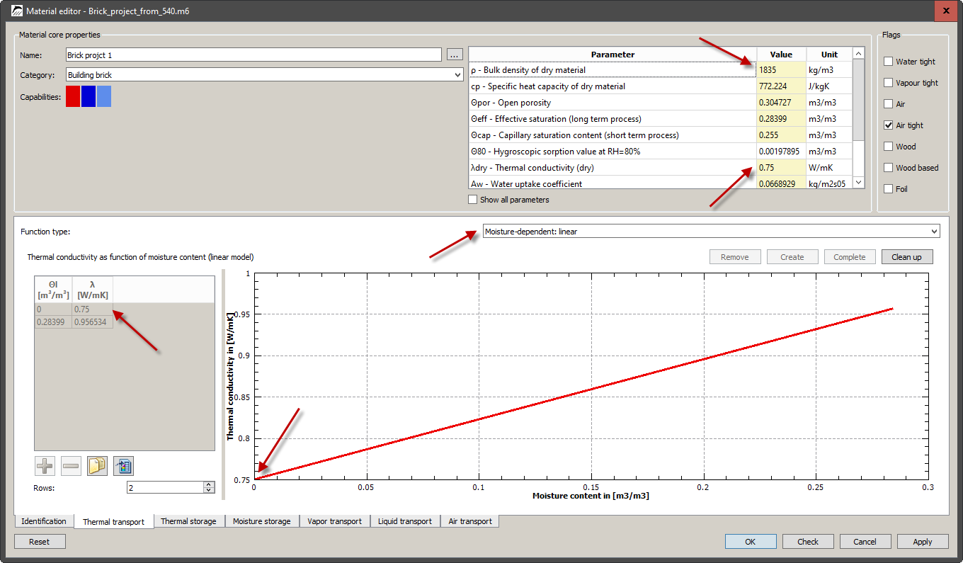
The red arrows point to the changed data.
The next step is to switch to liquid water transport section. Here a function Kl(Θl) is specified as data pairs. There is also a Kl_Eff value in the basic parameters. Therefore an adjustment by means of the Aw-value is possible. The figure below shows the result.
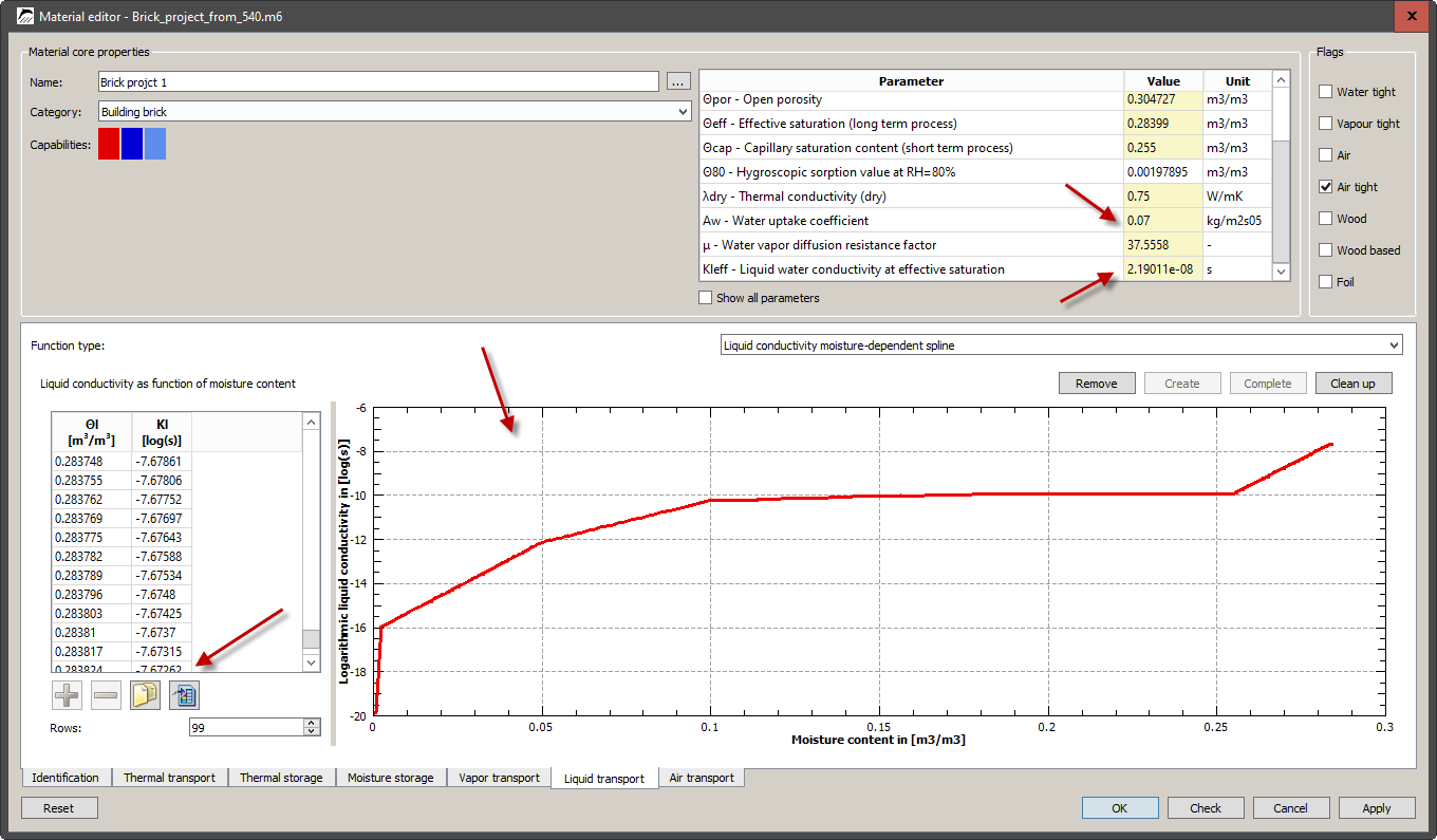
The changes are now complete and the material can be used. A click on Check shows the current status of the material.
Since no characteristic values for vapour transport were measured in the present case, uncertainties regarding the correctness may arise. If a measurement is not possible, at least a sensitivity study should be performed. This means creating variants of the material with different μ-values and comparing the results. If these do not differ greatly, it means the vapour diffusion of this brick has little effect. Then no further considerations are necessary. If the differences are large, however, further material measurements should be made. To create variants, proceed as follows:
-
Copy of the material to be changed
-
In the reference dialog that appears, duplicate the material file
The name of the new material file and also the new material name should reflect the change. Then you can adjust the new material. This way you can create as many variations as you like. The figure below shows the new material list.
2.3. Make material permeable to air
A top floor ceiling under an unheated attic space is to be investigated. Severe moisture damage had occurred in the ceiling. It is assumed that this damage was caused by convective moisture flow. To illustrate this, the construction is to be calculated with air flow. The following figure shows the construction with the materials and the paths of the air flow.
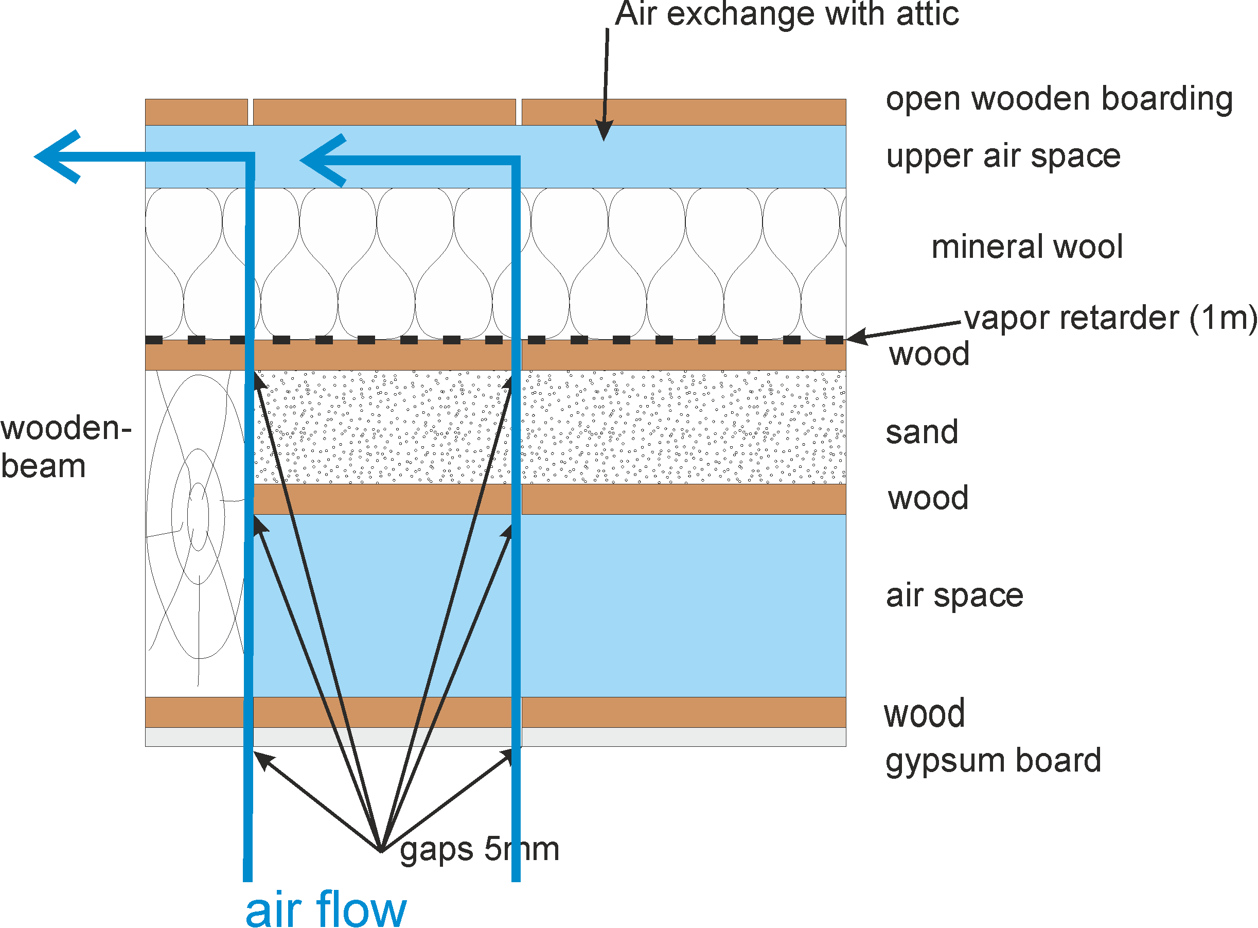
As can be seen in the figure, the air flow should flow from bottom to top through gaps in the wooden formwork, through the sand fill and the mineral wool into the upper air space. In order for DELPHIN to take air flow through materials into account, they must not be airtight and there must be a model for the (moisture-dependent) air permeability. For this, three materials have to be examined:
-
Air
-
Mineral wool
-
Sand
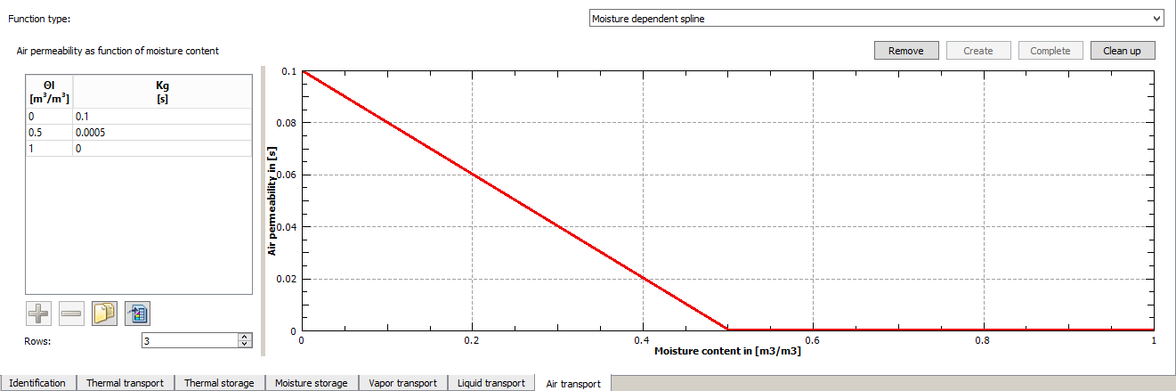
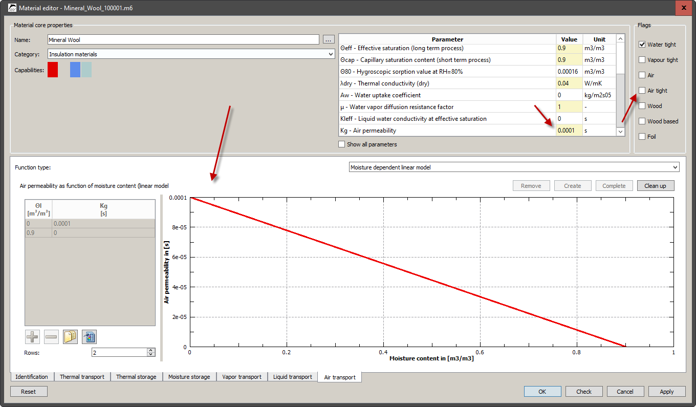
Air and mineral wool are both labelled as air permeable and have air permeability. As an example, the model for mineral wool is shown below.
The sand, on the other hand, is airtight and still needs to be adjusted. An additional task is that the air permeability for the sand should be independent of the moisture content. First, as explained in the other two examples, the material must be copied from the database into the project. Then the material editor for this material is called and the section Air transport is selected. The following display then appears.
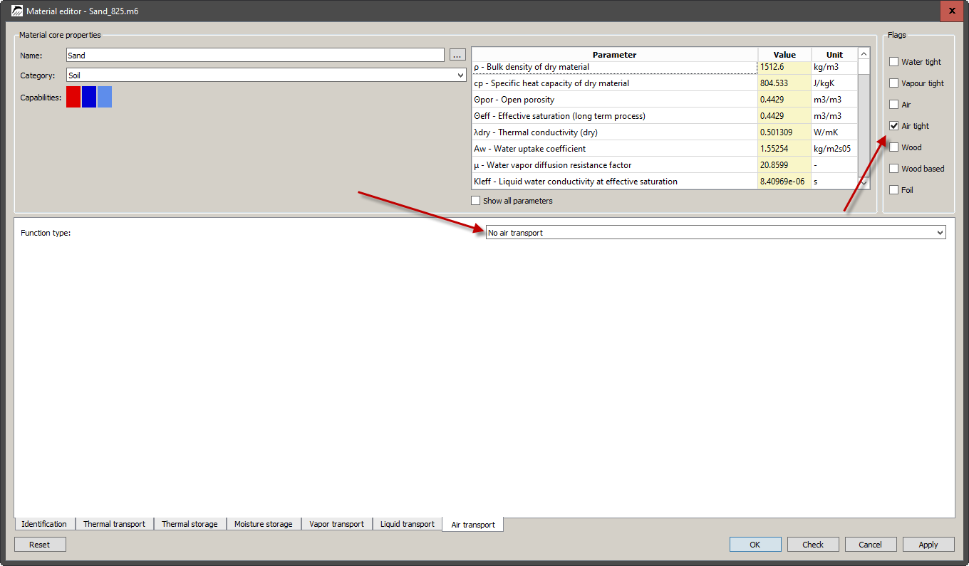
The following can be seen:
-
The flag for airtight is set (red arrow).
-
There is no model for air transport.
-
There is no basic parameter for air permeability.
First the flag for air tightness is switched off. Then the basic parameter list is extended so that the parameters that are not set are also visible. To do this, click on Show all parameters.
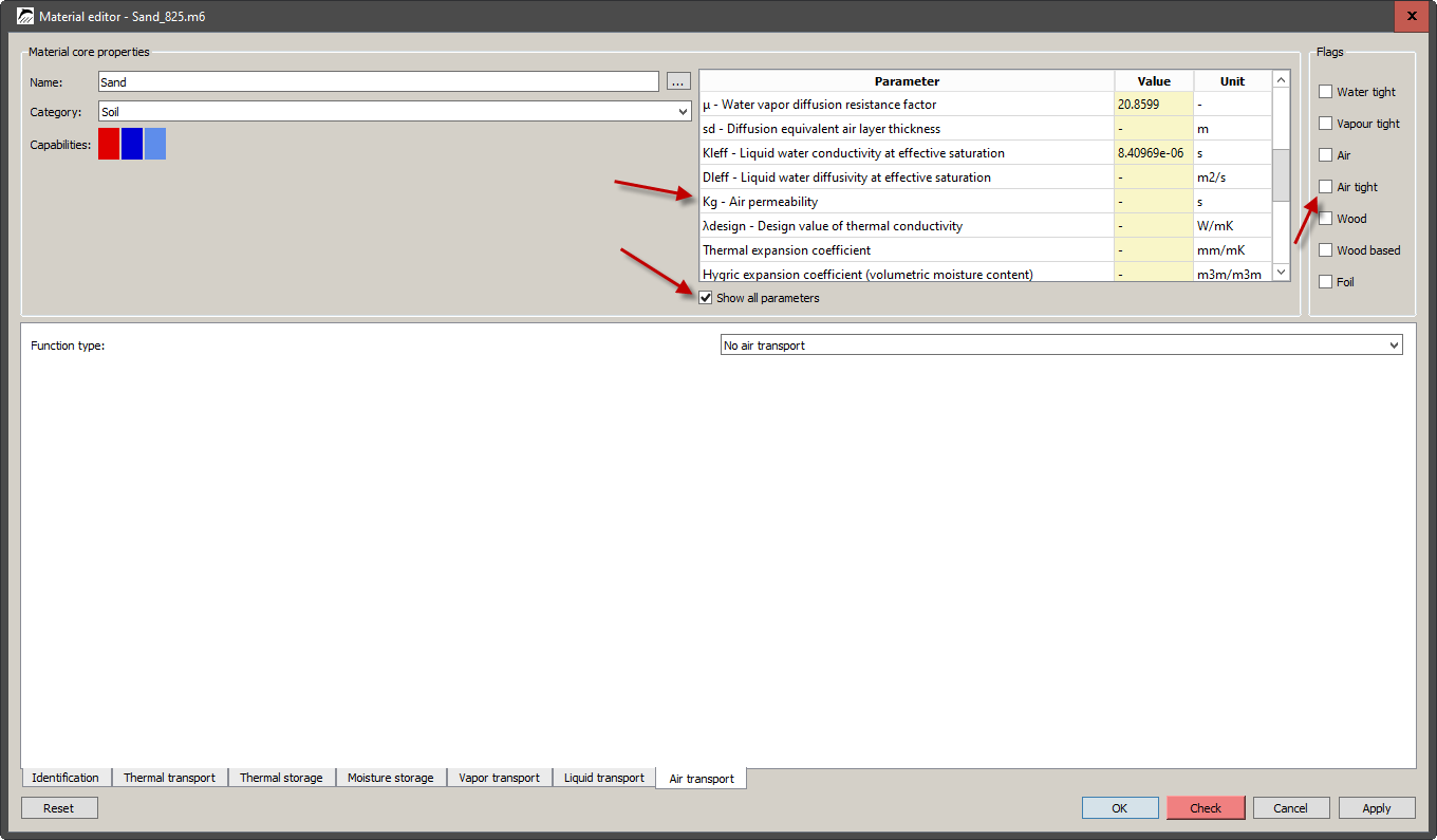
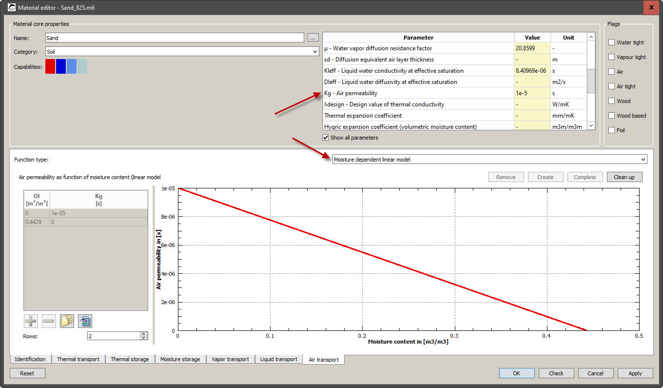
Immediately after switching off the airtightness flag, the Check button at the bottom turns red. This is the case because the material should now be able to calculate air transport, but no model exists yet. After checking Show all parameters the air permeability Kg is also shown in the basic parameter list (see picture above).
Next, a value for Kg is entered. Of course, this can only be an estimated value here, since no measurements are available. As a clue one can look at the mineral wool. There a value of 1e-4 s is entered. Since sand will certainly be denser, we choose a value of 1e-5 s. When this has been done, you should first choose Moisture dependent: linear when selecting the model.
As you can see in the picture below, we now have a valid model. You can see this by the fact that the Check button is no longer red and the material is therefore valid.
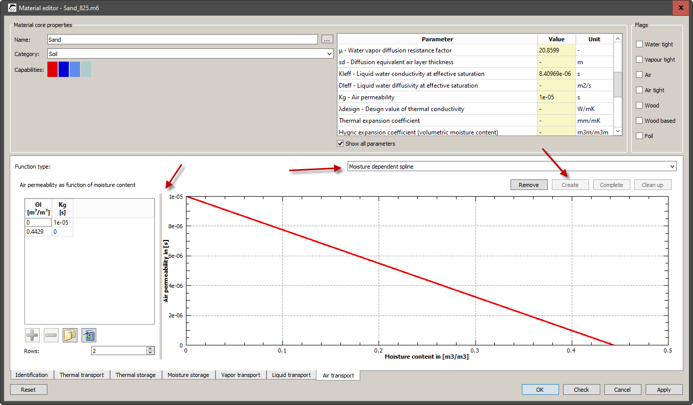
The simple linear model only requires air permeability and porosity and is therefore already valid here. However, the task states that for this material the air permeability should be independent of the moisture content. This is not yet the case. For this we need the other model Moisture dependent: Spline.
When you switch to it, the model view is empty for the time being. To create the model, you have to click on Create. Then a default data set is inserted. This corresponds to the linear model (see picture below).
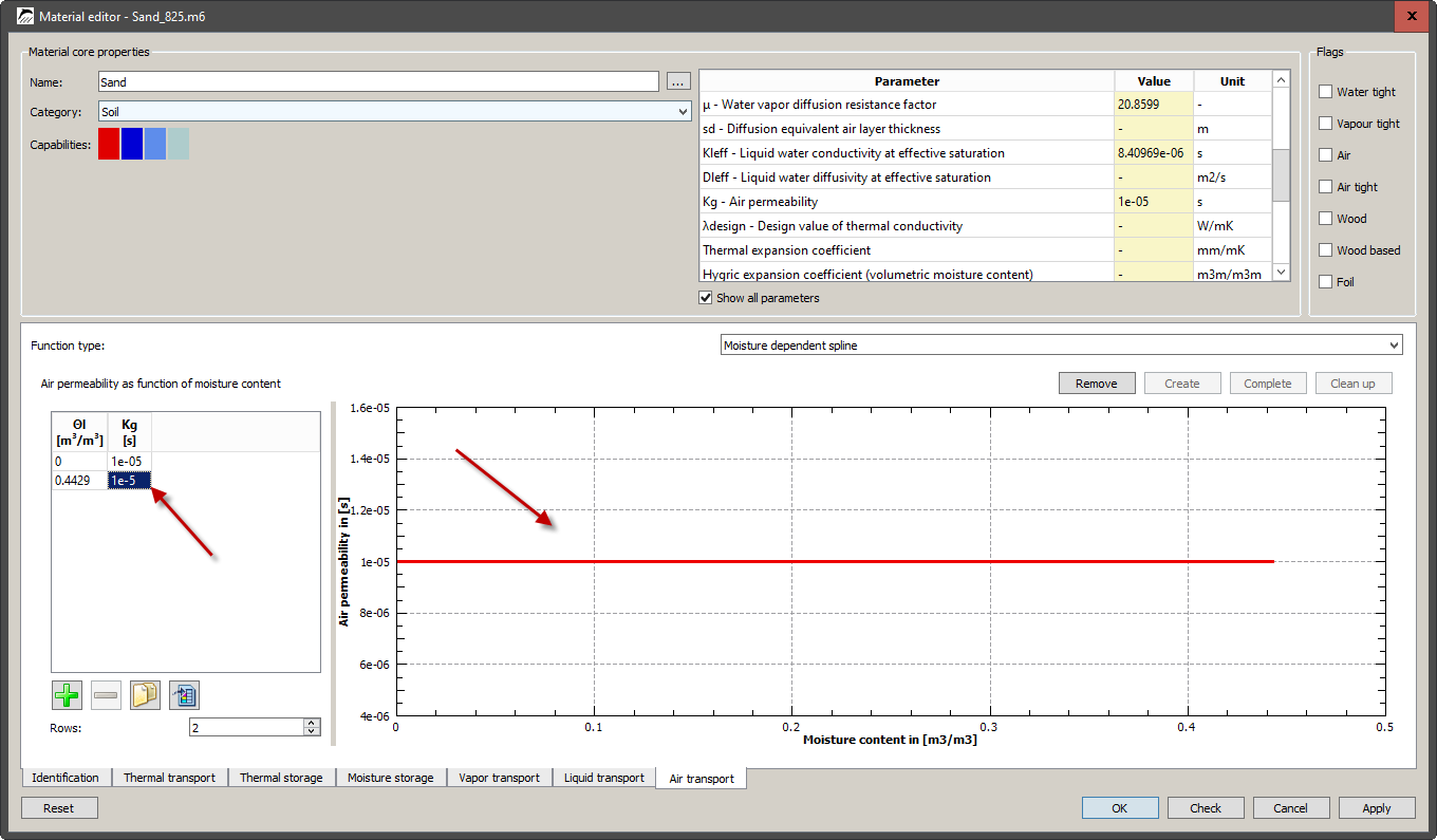
In contrast to the linear model, the data table is now editable. To remove the moisture dependence, only the Kg value for porosity must have the same value as for dry material. A double click on the value in the table opens the edit mode. The lower picture shows the final result.
The material can now be used. It would be conceivable here to create variants with different air permeabilities to investigate the influence of this value.